Giving this a shot using statsmodel’s tsa seasonal_decompose. Perhaps using this on stock market data would interest more people?
In any case, here is NYC’s Taxi Data from Numenta: https://www.kaggle.com/boltzmannbrain/nab/data
I broke it down into several timeframes for different perspectives.
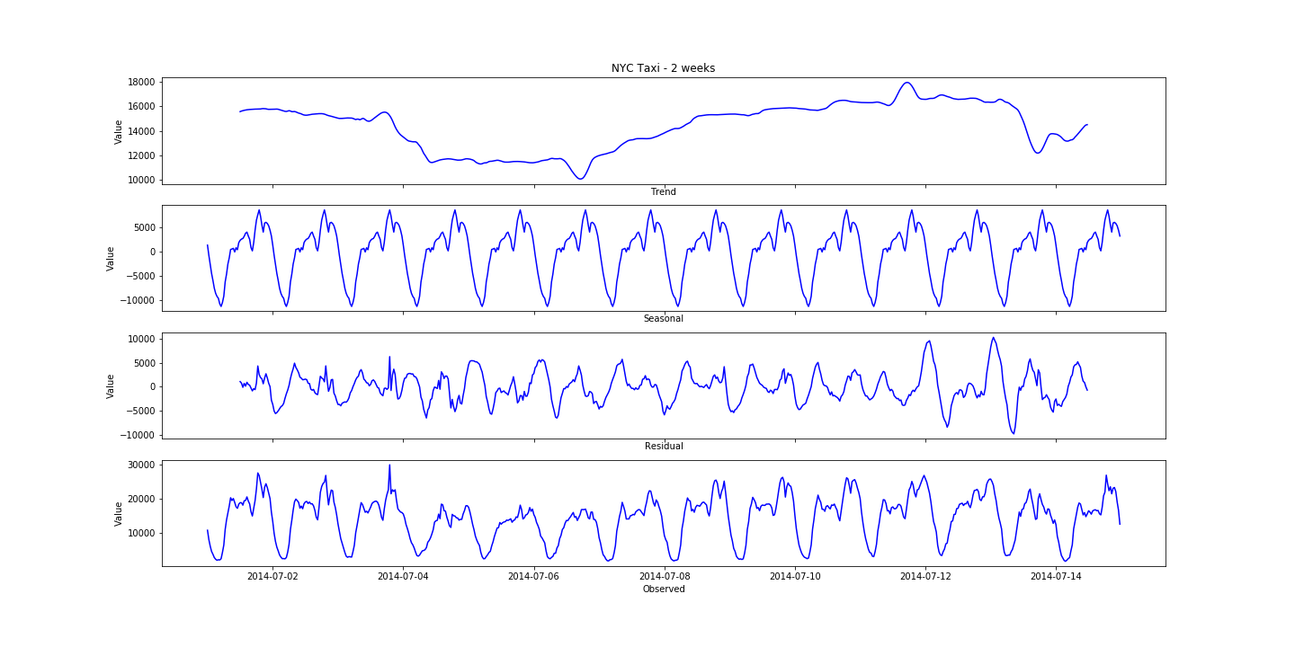
2 weeks’ worth of data:
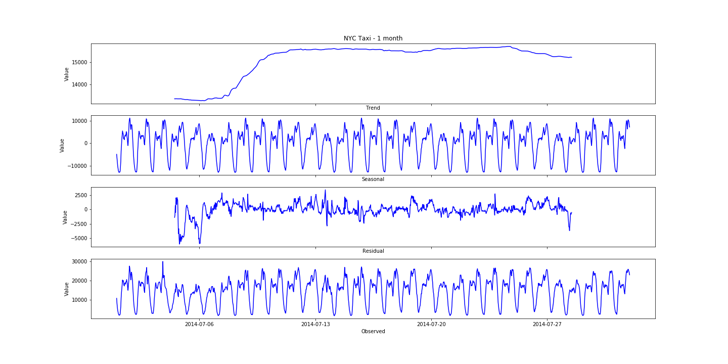
1 month’s worth of data:
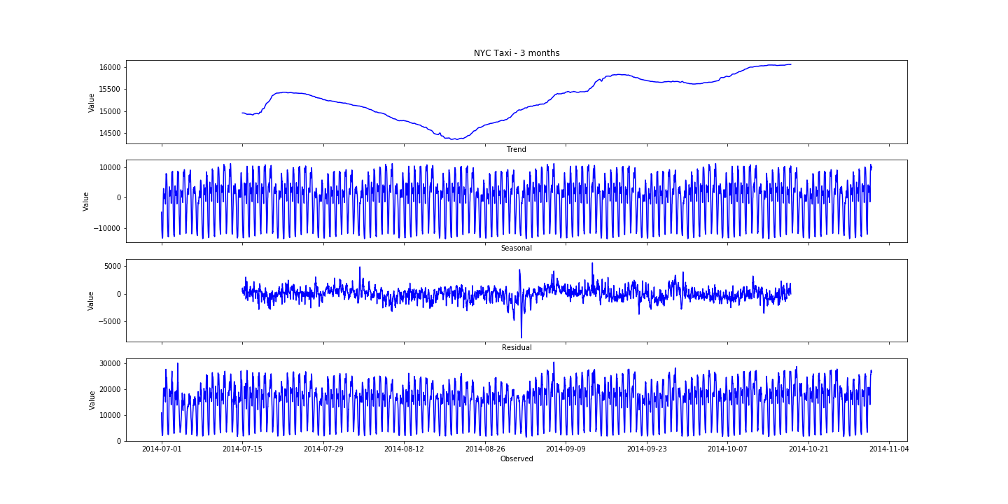
3 months’ worth of data:
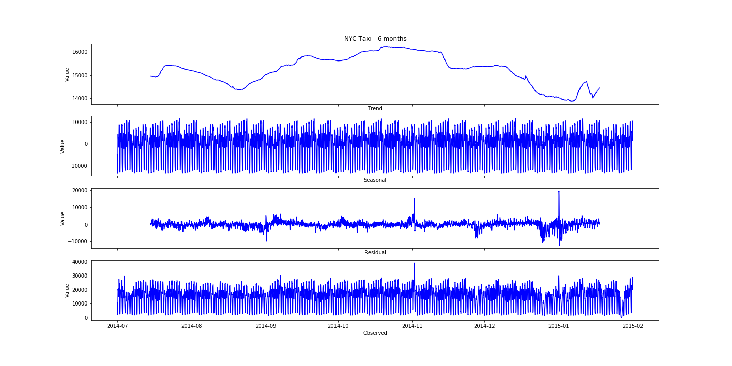
6 months’
import pandas as pd
import numpy as np
from statsmodels.tsa.seasonal import seasonal_decompose
import matplotlib.pyplot as plt
%matplotlib inline

# import data
taxi_6mths = pd.read_csv('nyc_taxi.csv')

# split into various timeframes
taxi_3mths = taxi_6mths[:5904]
taxi_1mth = taxi_3mths[:1488]
taxi_2wks = taxi_1mth[:672]

# define function to model and plot each dataframe
def decomp(df, freq, title):
    result = seasonal_decompose(df.value.values, freq=freq)
    results_df = pd.DataFrame({'trend': result.trend, 'seasonal': result.seasonal, 'resid': result.resid, 'observed': result.observed})
    df['timestamp'] = pd.to_datetime(df['timestamp'])

    # plot the graphs
    f, ax = plt.subplots(4, 1, sharex=True, figsize=(20, 10))

    ax[0].plot(df['timestamp'], results_df['trend'], 'b')
    ax[0].set_title(title)
    ax[0].set_xlabel('Trend')
    ax[0].set_ylabel('Value')

    ax[1].plot(df['timestamp'], results_df['seasonal'], 'b')
    ax[1].set_xlabel('Seasonal')
    ax[1].set_ylabel('Value')

    ax[2].plot(df['timestamp'], results_df['resid'], 'b')
    ax[2].set_xlabel('Residual')
    ax[2].set_ylabel('Value')

    ax[3].plot(df['timestamp'], results_df['observed'], 'b')
    ax[3].set_xlabel('Observed')
    ax[3].set_ylabel('Value')

    plt.savefig(f'{title}.png')


# run for each timeframe
decomp(taxi_6mths, 2*24*7*4, 'NYC Taxi - 6 months') # the time data given is at 30minute intervals
decomp(taxi_3mths, 2*24*7*4, 'NYC Taxi - 3 months')
decomp(taxi_1mth, 2*24*7, 'NYC Taxi - 1 month')
decomp(taxi_2wks, 2*24, 'NYC Taxi - 2 weeks')